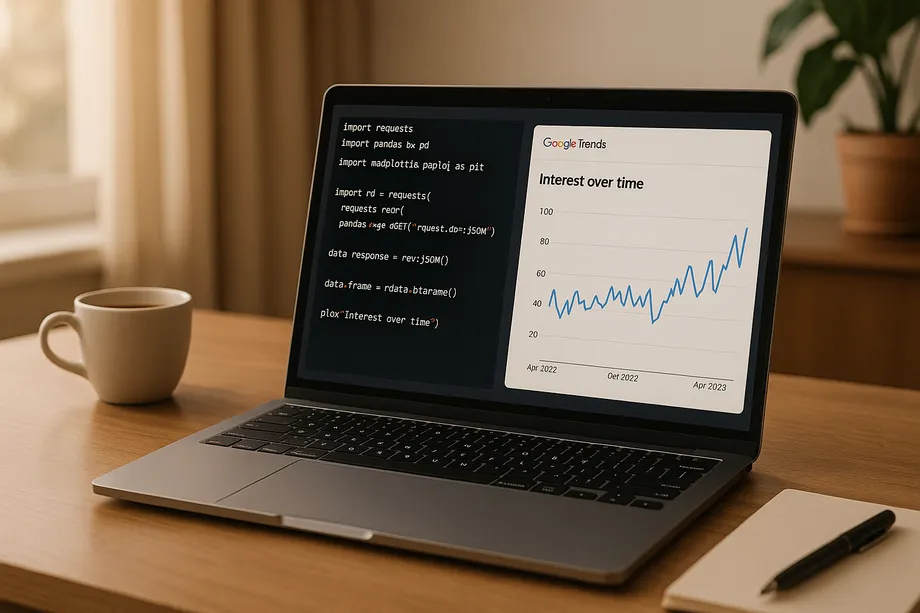
How to Scrape Google Trends with Python?

Want to analyze search trends and consumer behavior using Google Trends data? Python makes it easy to automate data collection and uncover insights. Here's what you need to know:

• Why Google Trends? It provides real-time and historical search data, showing interest levels for specific terms over time and by location.
• Why Python? Python's libraries like PyTrendssimplify data extraction, analysis, and visualization at scale.
• Legal Considerations: Scraping public data is generally legal in the U.S., but ensure compliance with Google's Terms of Service and privacy laws.

Steps to Get Started:

1. Set Up Python Environment: Install libraries like PyTrends, Pandas, and Matplotlib.
2. Use PyTrends: Automate data collection with methods like interest_over_time() and interest_by_region().
3. Process Data: Clean, organize, and export data in formats like CSV or JSON.
4. Visualize Trends: Use Matplotlib to create charts for easy interpretation.
5. Scale with Automation: Use proxies and scheduling tools for large-scale data collection.

By following these steps, you can use Google Trends data to monitor market trends, improve marketing strategies, and make data-driven decisions.

Setting Up Your Python Environment

Once you’ve got your legal and strategic bases covered, it’s time to set up your Python environment for scraping Google Trends effectively. This involves installing the right tools and configuring your environment to ensure smooth data collection.

Installing Required Libraries

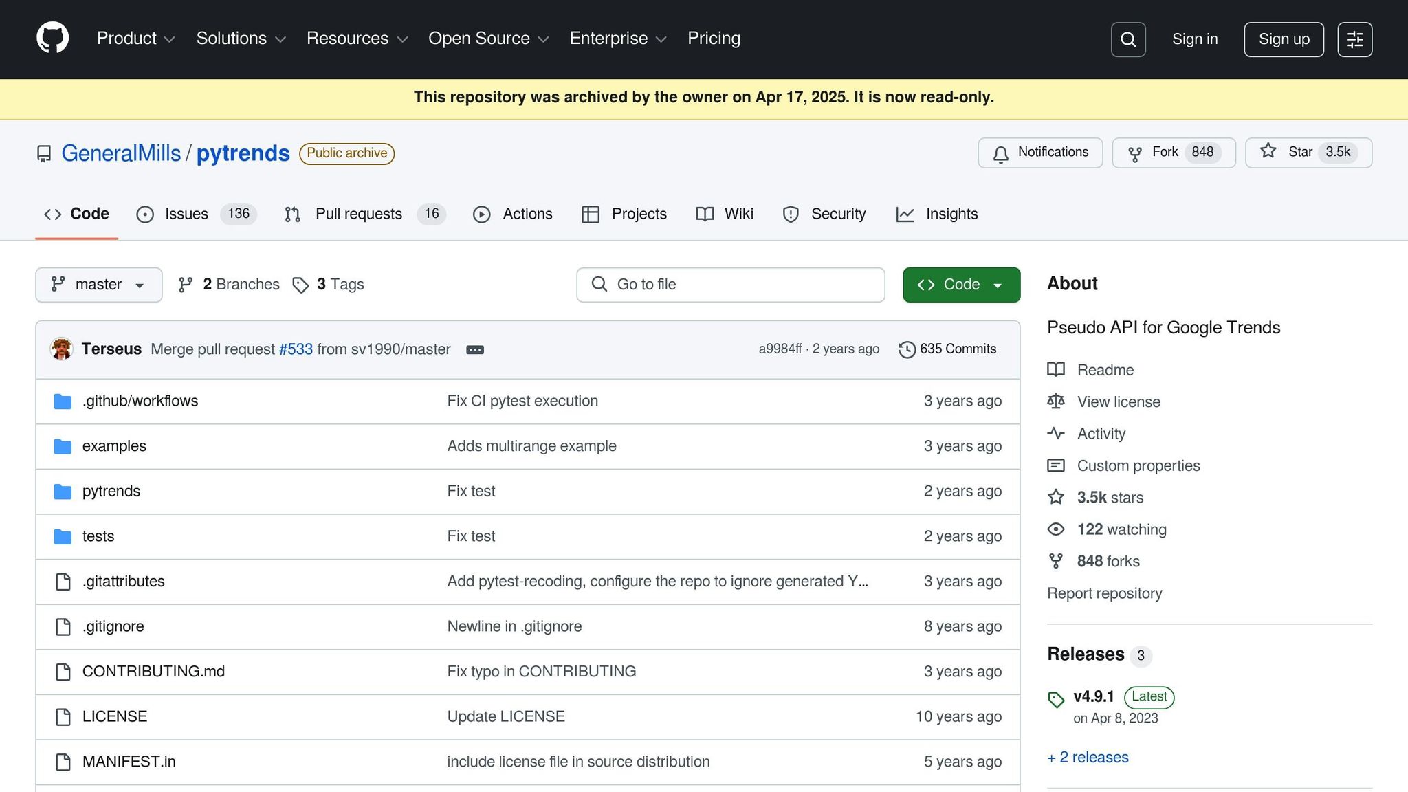
To get started, you’ll need to install a few essential Python libraries. The core tool for this task is PyTrends, which acts as an unofficial API for automating Google Trends data extraction.

PyTrends relies on other libraries to function seamlessly. For example:

• Requests manages HTTP communication with Google’s servers.
• lxml processes XML and HTML data.
• Pandas and Matplotlib handle data analysis and visualization.

It’s a good idea to create a virtual environment to keep your project dependencies organized. Run the following command to set one up:

python -m venv env

Then activate it:

• On Windows: env\Scripts\activate
• On macOS/Linux: source env/bin/activate

Once your virtual environment is active, install the required packages with these commands:

• pip install pytrends
• pip install pandas
• pip install matplotlib
• pip install lxml

While PyTrends will automatically install most of its dependencies, installing Pandas and Matplotlib separately ensures you’re working with the latest versions, which is crucial for robust data analysis and visualization.

Setting Up PyTrends Authentication

After installing the necessary libraries, you’ll need to configure PyTrends for collecting data tailored to the US market. The TrendReq object is your main tool for connecting to Google Trends, and setting it up correctly is key to reliable data extraction.

Here’s how you can initialize the TrendReq object:

from pytrends.request import TrendReq

pytrends = TrendReq(hl='en-US', tz=360)

In this example:

• hl='en-US' ensures that Google Trends returns data formatted for English-speaking users in the US.
• tz=360 sets the timezone to US Central Standard Time. You can adjust this value depending on your specific region.

This setup ensures that the data you collect aligns with American market expectations, including proper date formatting and regional context.

Configuring Settings for US Data

To focus on US-specific trends, you’ll need to adjust certain geographic and formatting parameters. These settings ensure the data you scrape accurately reflects American consumer behavior.

• Geographic Filtering: Use geo='US' in your data payload to filter results specifically for the United States. This is essential for businesses targeting domestic trends.
• Trending Searches: To get a list of trending searches in the US, use the trending_searches method with pn='united_states'. This will return a Pandas DataFrame with the most popular search queries among US users.
• Real-Time Trends: For real-time data, use the realtime_trending_searches method with pn='US'.

Additionally, make sure your system is configured to handle dates in the MM/DD/YYYY format, as this is the standard in the US. This consistency is important for generating reports that are easy to interpret across teams and stakeholders.

If you want to dive deeper into regional trends, you can specify individual states or metropolitan areas in your payload. This allows you to analyze how trends vary between regions like New York, California, or Texas.

Collecting Google Trends Data with PyTrends

With your environment set up, it’s time to dive into collecting data using PyTrends. This tool offers several methods to pull Google Trends data tailored for different types of analysis. Knowing how to use these methods effectively ensures you can gather the data you need for research or business insights.

Getting Historical Trend Data

The interest_over_time() method is your go-to for retrieving historical search data. It provides a timeline showing when specific keywords were most frequently searched.

Before using this method, you need to build a payload. Pay special attention to the timeframe parameter, which defines the range of your data. You can use formats like "today 5-y" for the past five years or specify exact dates, such as "YYYY-MM-DD YYYY-MM-DD".

Here’s an example of how to pull data for "Cloud Computing" over the last 12 months:

from pytrends.request import TrendReq
import pandas as pd

pytrends = TrendReq(hl='en-US', tz=360)
kw_list = ['Cloud Computing']
pytrends.build_payload(kw_list, cat=0, timeframe='today 12-m', geo='US')
df = pytrends.interest_over_time()

This code returns a DataFrame showing search interest for "Cloud Computing" in the US over the past year. The values are relative: 100 represents peak popularity, 50 means half as popular, and 0 indicates not enough data.

For more detailed analysis, you can use the get_historical_interest() method to gather hourly data. However, note that this method retrieves one week of hourly data per request, so you may need multiple API calls for extended timeframes:

pytrends.build_payload(kw_list, cat=0, timeframe='2024-01-01 2024-02-01', geo='US')
df = pytrends.interest_over_time()

To avoid hitting rate limits, insert delays between API calls using the sleep parameter. A 60-second delay is usually sufficient to prevent being blocked.

Getting Trends by Location

If you’re looking to analyze how search trends differ by region, the interest_by_region() method is your best bet. This function provides a geographic breakdown of search interest, making it invaluable for regional marketing or localized research.

The resolution parameter lets you control the level of detail. Options include 'CITY', 'COUNTRY', 'DMA' (metropolitan areas), and 'REGION'. For research focused on the US, 'DMA' is particularly useful for getting metro-level insights.

Here’s how to analyze search trends for major tech companies across US states:

pytrends = TrendReq(hl='en-US', tz=360)
kw_list = ['Facebook', 'Apple', 'Amazon', 'Netflix', 'Google']
pytrends.build_payload(kw_list=kw_list, geo='US')
df = pytrends.interest_by_region(resolution='REGION')

This returns data showing how search interest for these companies varies by state. The values range from 0 to 100, where 100 represents the region with the highest search volume relative to all searches in that area.

For more detailed insights, you can include regions with lower search volumes using inc_low_vol=True or add ISO codes for locations with inc_geo_code=True. If you’re targeting specific states, use the geo parameter (e.g., 'US-CA' for California or 'US-TX' for Texas).

Finding Related Search Terms

Uncovering related keywords can significantly enhance your market research or content strategy. PyTrends offers two methods for this: related_queries() and suggestions().

• related_queries(): This method identifies search terms closely linked to your primary keyword. For instance, querying "machine learning" might return related searches like "what is machine learning" or "machine learning model." These results help you understand the broader context of your target keyword.

  pytrends.build_payload(['machine learning'], geo='US')
  related_queries = pytrends.related_queries()
  

• suggestions(): This method provides keyword suggestions directly from Google Trends. For example, searching for suggestions related to "Business Intelligence" might return terms like "Business Intelligence Software" or "Market Intelligence."

  suggestions = pytrends.suggestions(keyword='Business Intelligence')
  

With this data in hand, you’re ready to move on to cleaning, saving, and visualizing the results in the next steps.

Processing and Displaying Your Data

Building on the earlier discussion about data collection, this section focuses on turning your raw Google Trends data into meaningful business insights through proper processing, storage, and visualization techniques.

Cleaning and Organizing Data

When working with Google Trends data, the PyTrends DataFrame index contains datetime objects. For US-specific business reporting, these need to be converted into the MM/DD/YYYY format:

import pandas as pd
from datetime import datetime

# Convert the datetime index to US date format
df.index = pd.to_datetime(df.index)
df['Date'] = df.index.strftime('%m/%d/%Y')

To better understand long-term trends, group data into monthly or quarterly summaries. This reduces short-term noise and highlights broader patterns, aligning with common US business cycles. Additionally, calculating percentage changes over specific periods can offer insights into growth or decline:

# Calculate month-over-month percentage changes
df['Monthly_Change'] = df['search_term'].pct_change(periods=4) * 100

Rows with incomplete or zero data should be removed unless they represent meaningful anomalies. Data validation is also critical - watch for unusual spikes that could result from collection errors or one-time events. Clean and organized data is the foundation for reliable analysis and seamless integration with business tools.

Saving Data for Business Use

Once your data is processed, exporting it in formats suitable for your business systems is essential. CSV files are a versatile choice for spreadsheets and databases:

# Export with US-friendly formatting
df.to_csv('google_trends_data.csv', 
          date_format='%m/%d/%Y',
          float_format='%.2f')

For web applications or APIs, JSON is a better option as it preserves data types and nested structures:

import json

# Convert DataFrame to JSON with proper formatting
json_data = df.to_json(orient='records', date_format='iso')
with open('trends_data.json', 'w') as f:
    json.dump(json.loads(json_data), f, indent=2)

Excel Power Query is another great tool for cleaning and transforming Google Trends data directly within Excel. It can automate repetitive tasks and create refreshable links to your Python-generated CSV files.

To keep your data archives organized, adopt a standardized naming convention. For example, a file named trends_cloud_computing_01012024_12312024.csv clearly indicates the topic and date range.

Exporting your cleaned data in widely compatible formats ensures smooth integration with your business systems. Once that's done, the next step is to bring the data to life with visualizations using Matplotlib.

Making Charts with Matplotlib

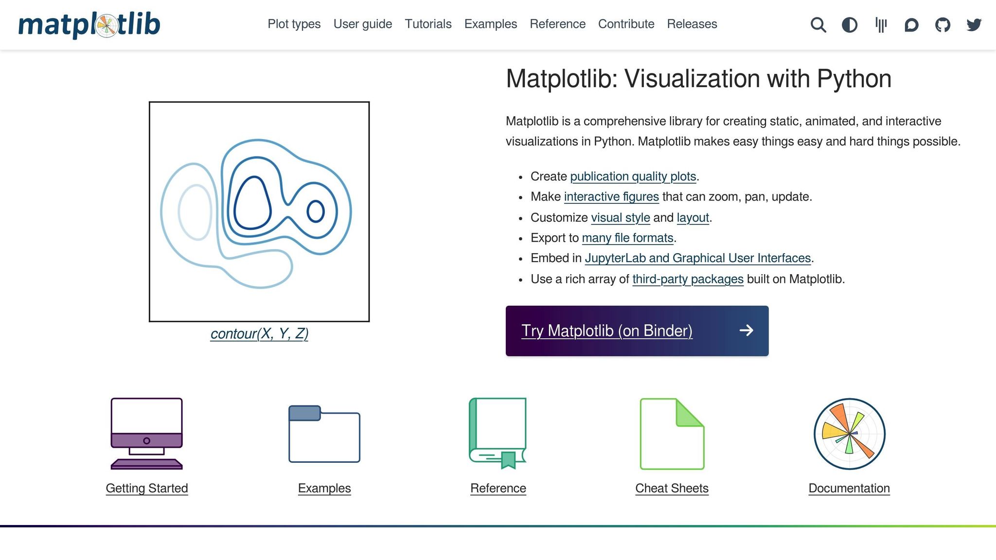
Visualizing your Google Trends data is key to uncovering insights. Matplotlib offers powerful tools to turn raw data into clear, impactful charts.

For example, you can create a professional line chart to showcase search interest trends over time:

import matplotlib.pyplot as plt
import matplotlib.dates as mdates

# Create a professional-looking line chart
fig, ax = plt.subplots(figsize=(12, 6))
ax.plot(df.index, df['keyword'], linewidth=2, color='#1f77b4')
ax.set_title('Search Interest Over Time', fontsize=16, fontweight='bold')
ax.set_xlabel('Date', fontsize=12)
ax.set_ylabel('Search Interest (0-100)', fontsize=12)

# Format dates for US audiences
ax.xaxis.set_major_formatter(mdates.DateFormatter('%m/%d/%Y'))
ax.xaxis.set_major_locator(mdates.MonthLocator(interval=3))
plt.xticks(rotation=45)

To maintain a polished look, use a consistent color palette that matches your company’s branding. Avoid using more than 5-6 colors in any chart to keep the visual focus clear.

For comparing regional data, horizontal bar charts work well:

# Create horizontal bar chart for regional data
fig, ax = plt.subplots(figsize=(10, 8))
regions = df_regional.index[:10]  # Top 10 regions
values = df_regional.values[:10]

bars = ax.barh(regions, values, color='#2ca02c')
ax.set_title('Search Interest by State', fontsize=16, fontweight='bold')
ax.set_xlabel('Relative Search Interest', fontsize=12)

# Add value labels on bars
for i, bar in enumerate(bars):
    width = bar.get_width()
    ax.text(width + 1, bar.get_y() + bar.get_height()/2, 
            f'{width:.0f}', ha='left', va='center')

For presentations, light gray gridlines provide helpful reference points without overpowering the data. If you're creating multiple charts for the same report, ensure consistent scaling and formatting to make comparisons easier. Always save your charts in high-resolution formats (300 DPI) for professional printing and presentations.

sbb-itb-65bdb53

Large-Scale Data Collection and Automation

Scraping Google Trends data at an enterprise level is no small feat. Manually gathering data quickly becomes unmanageable when your business requires thousands of queries daily. To meet these demands, automation tools and strategies are essential. Below, we’ll explore methods for scaling your data collection efforts, from proxy management to fully automated systems and professional services.

Using Proxy Servers

Google Trends imposes limits on high-frequency queries, often blocking IP addresses that send too many requests. For businesses operating at scale, proxy servers are crucial. By rotating proxies with fresh IP addresses, you can query multiple topics or timeframes without triggering Google’s defenses. A recommended approach is to space requests by three to five seconds to minimize suspicion.

Residential proxies are especially effective for scraping Google Trends. These proxies use IP addresses tied to real users, making them less likely to be flagged by Google’s systems.

Here’s a simple Python example for rotating proxies during data collection:

import requests
from itertools import cycle
import time

# Proxy rotation setup
proxies = [
    {'http': 'http://proxy1:port', 'https': 'https://proxy1:port'},
    {'http': 'http://proxy2:port', 'https': 'https://proxy2:port'},
    {'http': 'http://proxy3:port', 'https': 'https://proxy3:port'}
]
proxy_cycle = cycle(proxies)

# Collect data using rotating proxies
for keyword in keyword_list:
    current_proxy = next(proxy_cycle)
    response = requests.get(trends_url, proxies=current_proxy)
    time.sleep(4)  # Pause between requests

Geo-targeted proxies can also be used to access location-specific Google Trends data. For example, these proxies allow you to analyze trends in the U.S. versus trends in other regions. To further enhance stealth, combine proxy rotation with headless browsers like Puppeteer or Selenium. While datacenter proxies are faster, residential proxies provide better long-term reliability for avoiding detection.

Setting Up Automated Data Collection

Proxies solve the problem of high-frequency requests, but automation takes your data collection to the next level. Tools like Playwright and Selenium allow you to simulate user interactions with the Google Trends interface, automating actions such as searching for terms and downloading CSV files.

Here’s an example of using Playwright to automate Google Trends data collection:

from playwright.sync_api import sync_playwright
import schedule
import time

def automated_trends_collection():
    with sync_playwright() as p:
        browser = p.chromium.launch(headless=True)
        page = browser.new_page()

        # Open Google Trends and search for a keyword
        page.goto("https://trends.google.com/trends/")
        page.fill('input[placeholder="Enter a search term or a topic"]', keyword)
        page.press('input[placeholder="Enter a search term or a topic"]', 'Enter')

        # Wait for results and download the CSV
        page.wait_for_selector('.widget-actions')
        page.click('button[aria-label="Download CSV"]')

        browser.close()

# Schedule daily data collection
schedule.every().day.at("09:00").do(automated_trends_collection)
schedule.every().day.at("15:00").do(automated_trends_collection)

while True:
    schedule.run_pending()
    time.sleep(60)

To handle potential issues like rate limits (HTTP 429 errors), implement retry logic with exponential backoff. This approach ensures your system waits longer between retries, reducing the risk of permanent blocks:

import random

def retry_with_backoff(func, max_retries=5):
    for attempt in range(max_retries):
        try:
            return func()
        except Exception as e:
            if attempt == max_retries - 1:
                raise e
            wait_time = (2 ** attempt) + random.uniform(0, 1)
            time.sleep(wait_time)

Scheduling your scripts during off-peak hours, like early mornings (6:00 AM EST) or late evenings (10:00 PM EST), can also help avoid server restrictions.

Using Professional Data Services

If managing proxies, scripts, and automation feels overwhelming, professional data services can simplify the process. Providers like Web Scraping HQ offer complete solutions for extracting Google Trends data. These services handle everything from proxy management to anti-bot detection, delivering clean, structured data directly to your team.

For example:

• Standard Plan ($449/month): Includes ready-to-use Google Trends data, automated quality checks, and expert support.
• Custom Plan (starting at $999/month): Offers tailored data formats, enterprise-level service agreements, and priority support with 24-hour delivery.

Given that Google Trends usage has surged by 80% for decision-making purposes, outsourcing this task can save time and resources. Professional services also ensure compliance with Google’saterms of service, reducing legal risks while maintaining data accuracy.

For businesses tracking hundreds of keywords across multiple regions, these managed services often prove more cost-effective than maintaining internal scraping teams and infrastructure. Whether you choose to build your own system or rely on external providers, the key is having the right tools and processes in place to harness the full potential of Google Trends data.

Summary and Next Steps

Key Insights on Using Google Trends Data with Python

Using Python to scrape Google Trends data can unlock valuable insights for businesses in the United States. By leveraging Python's tools and automation capabilities, you can collect search interest data across various timeframes and geographic regions. This method offers a fresh perspective on consumer behavior and market patterns.

Python simplifies the process by automating the extraction of large volumes of search data. Considering that Google processes over 1 billion searches daily, the information available for analysis is immense. However, it's essential to stay within legal boundaries by adhering to Google's terms of service and data privacy regulations. Transparency in how data is used fosters trust with both customers and stakeholders.

While building your system offers flexibility, scaling up often requires external support to handle the challenges of large-scale data collection.

Why Consider Web Scraping HQ Services?

Creating a custom Google Trends scraping setup can be a great learning experience, but for enterprise-scale operations, professional services often make more sense. Web Scraping HQ simplifies the complexities of managing proxies, rate limits, and anti-detection systems.

Their Standard Plan, priced at $449/month, offers structured data with automated quality checks and expert support. This eliminates the need for maintaining scripts, ensuring accurate data and compliance with legal standards. For businesses tracking hundreds of keywords across multiple U.S. regions, this managed solution is often more cost-efficient than maintaining an in-house team.

For larger needs, custom plans starting at $999/month provide enterprise-level support. These include scalable infrastructure, flexible data schemas, and 24-hour delivery, ideal for companies running thousands of daily queries. With Google Trends usage increasing by 80% for decision-making, having a reliable data infrastructure is crucial for staying competitive.

Leverage your Python expertise for quick analysis and prototyping, but rely on managed services for large-scale data collection that supports critical business decisions. This balance ensures you get the best of both worlds: flexibility for exploration and reliability for production-level needs.