Car Rental Price Scraping: A Practical 2026 Guide

Most advice on car rental price scraping starts with the wrong field. A daily headline rate is easy to collect, easy to chart, and often inadequate for a buying decision. A production system that compares only the visible rate can make a vendor look cheaper while ignoring the charges that appear later in the reservation flow.

The practical problem is the quote-to-final-price gap. The UK Competition and Markets Authority described rental-car drip pricing as a pattern in which consumers weren’t made aware of all costs at reservation time and later faced additional charges at pickup, while the European Commission documented commitments covering mandatory charges, surcharges, optional extras, insurance products, fuel policies, and pre-authorisation requirements in its car-rental case study (CMA report on rental-car pricing transparency). A Which? survey of more than 3,600 consumers found that 13% said they paid more than the price first quoted, making quote capture across booking stages a foundational scraping requirement.

The rest of the pipeline should follow that buyer problem. Capture the offer, resolve its dimensions, preserve each cost component, and compare normalized totals rather than decorative daily rates.

Why Headline Rates Mislead Scraping Buyers

A scraper that collects only the lowest displayed daily rate can produce a polished, inaccurate market view. The base price may exclude location surcharges, taxes, protection products, mileage limits, fuel conditions, driver-age charges, or one-way fees. These items can change the payable amount without changing the headline rate.

The booking dimensions matter as much as the number. A quote for an airport pickup, a downtown branch, a short lead time, or unlimited mileage is not directly comparable with a quote using different conditions. Production pipelines should retain those dimensions before comparing vendors, then capture the price again at the latest reliable stage of the reservation flow. The CMA evidence on drip pricing and additional rental charges supports treating later-disclosed charges as a data-capture problem, not a minor presentation detail.

An aggregator that exposes only the base rate can support discovery. It cannot support dependable cost benchmarking until the downstream fee stack and commercial terms are available. Traveler-focused material, including these Approved Experiences traveler car rental insights, can clarify booking context, but the pipeline still has to verify what each displayed price includes.

Practical rule: If analysts cannot reconstruct the payable total from stored fields, the scraped rate is not comparable enough for a pricing decision.

Headline-only data can create a false market signal. A low base rate may enter a report, forecast, or repricing workflow beside another vendor’s tax-inclusive total. The resulting difference then looks like competitive pricing rather than an incomplete quote. More scraping volume will not correct that defect. Repeatedly collecting the same incomplete field only produces more records that cannot support a fair comparison.

The cost stack buyers actually need

The following illustration is a normalization example, not a universal quote. It shows why the visible rate should not become the canonical field.

Rate Component	Amount (USD)	Notes
Headline daily rate	39	Displayed base rate
Mandatory and location charges	Not stated	Extract from the offer
Insurance or protection products	Not stated	Inclusion varies by vendor and market
Fuel and mileage terms	Not stated	Can change the effective trip cost
Final payable total	Not stated	Capture at the latest reliable booking stage

The useful unit of analysis is the all-in offer, not the isolated headline rate. Each record should preserve the original quote, pickup and return conditions, lead time, mileage and fuel rules, mandatory add-ons, and fee lines that explain how the total was formed. That structure supports normalization across markets while keeping the source offer auditable.

Designing the Schema That Captures All-In Cost

A production schema should make an offer reproducible. Start with identifiers that tell you exactly what was searched:

• Vendor: Store the rental company or aggregator name, plus the source page or endpoint class.
• Pickup and drop-off codes: Keep pickup_location_code and dropoff_location_code as separate fields. An airport branch and a downtown branch aren’t interchangeable products.
• Timestamps: Store pickup_datetime and return_datetime as ISO 8601 timestamps. Locale-formatted strings create avoidable ambiguity around dates, times, and time zones.
• Vehicle definition: Capture vehicle_class, transmission where exposed, passenger capacity where exposed, and the vendor’s own category label.
• Commercial terms: Preserve mileage_policy, currency, availability status, and any restrictions attached to the offer.

The pricing fields need equal attention. At minimum, store base_rate, insurance_options, taxes_and_fees, fuel_policy_charge, young_driver_fee, one_way_fee, location_surcharge, and total_quote. Add protection_options as structured data rather than burying the selection in free text. The system should also retain the raw response or a governed snapshot, because a parsed total without its source context is difficult to audit.

Separate inputs from derived values

Don’t combine pickup and drop-off into one string such as LAX to Downtown Los Angeles. Separate fields support route-level analysis, airport-versus-off-airport comparisons, and one-way fee reconciliation. The same principle applies to dates. A locale string can be parsed differently by different systems, while an ISO 8601 timestamp gives the pipeline a stable representation for lead-time calculations.

Store the breakdown alongside the total, not instead of it. Analysts may later want to compare tax-inclusive and tax-exclusive views, change the assumed protection package, or identify a newly introduced surcharge. A component-level record supports anomaly detection and reconciliation against confirmation emails or checkout captures.

A versioned schema prevents vendor changes from corrupting downstream outputs. When a site introduces a new mandatory line item, increment the schema version, preserve the unmapped field in raw data, and route the record to quality review. Teams building their own extraction stack can also use guidance on online web scraping services when deciding which collection and delivery components should remain managed rather than custom-built.

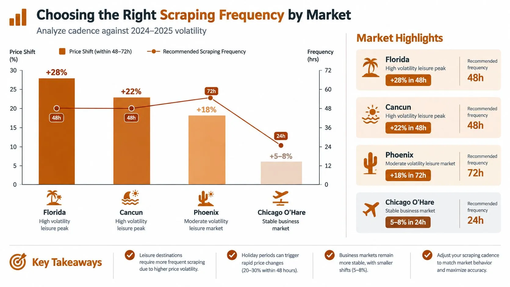
Choosing the Right Scraping Frequency by Market

Scraping frequency should follow inventory churn and all-in price movement, not a universal schedule. A practical starting point is 10 to 15 minutes for high-volatility markets and hourly collection for calmer ones, since daily snapshots can miss temporary changes (car rental price scraping cadence guidance). Apply that cadence to comparable pickup locations, lead times, mileage terms, and mandatory add-ons, rather than treating every airport as one market.

Recent monitoring suggests rental pricing has cooled from the extreme volatility earlier in the decade. North America’s average five-day rental price during June to September 2025 fell 13% year over year, while Europe kept a stronger seasonal summer peak (recent rental-car market monitoring). A separate market summary reported average rental prices declining from $347 per booking in March 2023 to about $291 in March 2025 across major markets. That pattern supports regional cadence decisions instead of high-frequency collection everywhere.

A cadence decision framework

• Sub-15-minute polling: Use it for high-velocity origin airports during holiday or event windows, when a short inventory change can alter the normalized offer.
• Hourly polling: Apply it to active leisure corridors where prices move often, but continuous browser sessions add cost without improving coverage.
• Daily polling: Use it for steadier business markets and long-running benchmarks, where location and vehicle coverage matter more than every intraday fluctuation.
• Event-triggered collection: Increase frequency when fleet scarcity, severe weather, major events, or unusual cancellation patterns signal a market shift.

Higher frequency raises request, proxy, and browser-automation consumption. It does not automatically improve decision quality. Track changes in the normalized total before fixing a schedule. If repeated intraday polls return the same result for a pickup location, lead time, vehicle class, and terms, slow that cell and spend capacity on combinations showing meaningful movement.

The useful question is which price or term changes would alter the decision, and how quickly the pipeline must detect them.

Working Through Anti-Bot and Access Layers

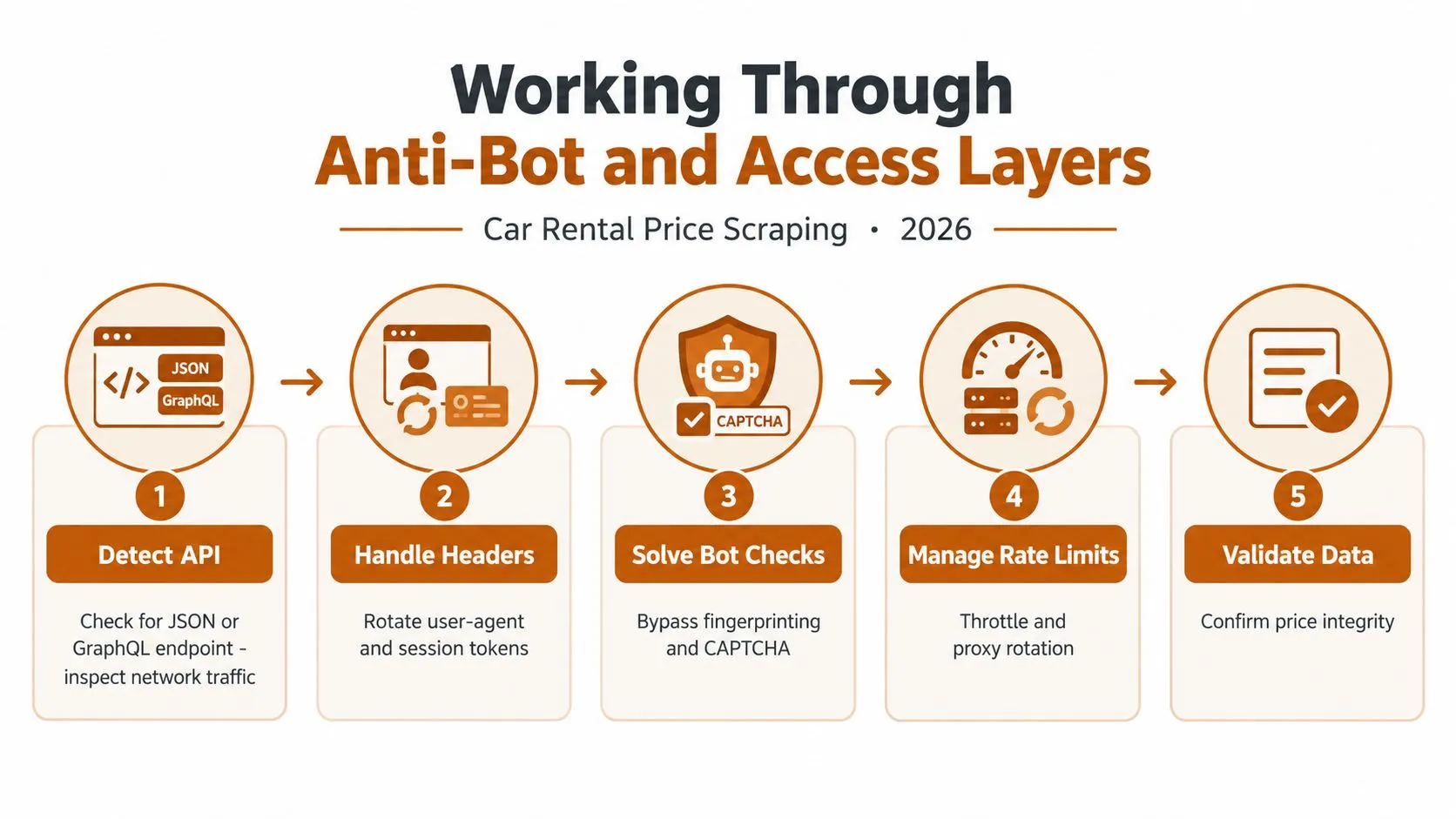
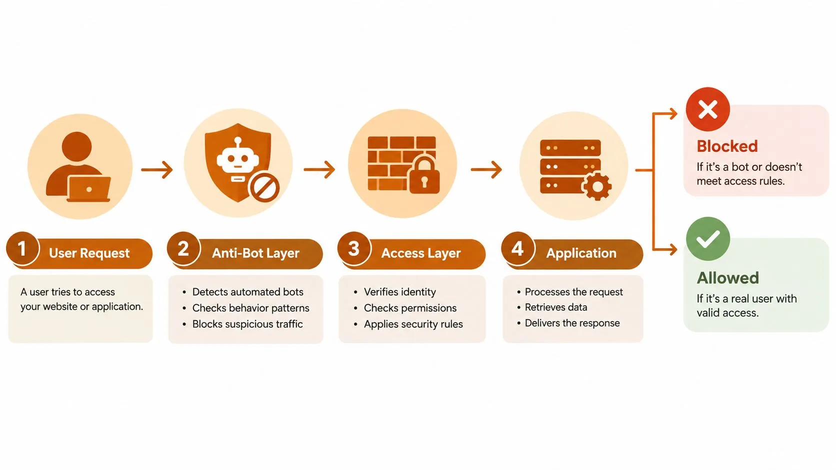
Anti-bot handling starts with the access path, not with a larger request pool. A browser session used for every search costs more and can expose a larger fingerprint than a controlled structured request. The target remains complete, verifiable rental data, including fees, availability, mileage terms, and mandatory add-ons.

Inspect the search flow and network traffic first. If the vendor returns JSON or GraphQL data behind the search widget, collect that response instead of parsing rendered HTML. Preserve the same session context, required headers, cookies, locale, currency, and request sequence. Keep parsers tolerant of optional fields. Public notes on car-rental scraping describe AWS WAF protection on RentalCars.com and the use of residential proxies for access, while a Turo-focused example combines a real browser with residential proxies around DataDome-protected flows (public car-rental scraper access notes).

Solve access problems in layers

1. Structured endpoint first: Identify the response containing offers, fees, availability, and rental terms.
2. Session consistency next: Maintain cookies, locale, currency, and search context across the full interaction.
3. Browser fallback: Use Playwright or Puppeteer only when interaction triggers rendering or a challenge requires browser execution.
4. Proxy and geography alignment: Match the exit region to the pickup market, language, currency, and timezone. Geolocation affects the quote itself.
5. Validation last: Compare results with a controlled route and flag unexpected changes in totals, currencies, fee structures, or offer counts.

A Frankfurt exit collecting Los Angeles airport results can receive a different market context and corrupt every comparison. Track CAPTCHA challenges, rate limits, fingerprint checks, and geolocation failures as separate metrics. The RETRO//STRESS bypass rate overview offers general background on bypass concepts, but rental collection still requires target-specific testing, authorization, and careful validation.

Use the guide to anti-bot measures in Playwright for implementation details. In production, choose the least complex method that returns the fields needed for all-in cost normalization. Escalate only when the source blocks or withholds those fields. More successful requests do not improve decisions if they produce headline rates without pickup context, lead time, mileage rules, or mandatory charges.

Planning the Request Matrix Across Vendors and Dates

A request matrix turns scraping from ad hoc sampling into explicit coverage. Each cell represents a combination of vendor, pickup location, drop-off location, date window, rental duration, vehicle class, and commercial assumptions. Without that enumeration, teams tend to over-collect familiar airport searches and miss the branches or lead times that explain the price difference.

Start by ranking sources by what they disclose. Tier one sources expose a complete or nearly complete cost breakdown. Tier two sources expose a partial quote and require add-on backfill or checkout verification. Tier three aggregators are useful for market discovery but may resell upstream inventory with different presentation or markup behavior. That ranking should influence both confidence scores and refresh investment.

For locations, include the airport branches and downtown branches that drive demand in the target market. Use stable airport codes where possible, because ambiguous city autocomplete can produce inconsistent availability. Expand dates across weekday, weekend, and holiday windows, then vary lead time across 1, 7, 14, 30, and 60 days as defined in the operating plan. Vehicle coverage should include at least economy, midsize, SUV, and luxury categories.

Coverage tiers

Tier	Vendors	Locations	Date Windows	Vehicle Classes	Cells per Cycle
Priority	Full all-in disclosure	Core airport and downtown branches	Weekday, weekend, holiday	Economy, midsize, SUV, luxury	Every defined combination
Standard	Partial disclosure with backfill	Core airport branches and selected off-airport branches	Weekday and weekend	Economy, midsize, SUV	Every defined combination where available
Discovery	Aggregators and variable sources	Broad market sample	Representative date windows	Main classes	Rotating sample with confidence flag

Naively expanding every dimension can make the request budget grow quickly. Use a coverage rule instead: every active cell must be filled at least once per cadence cycle, then assign refreshes according to observed volatility. High-variance cells stay on tighter rotation, while stable cells move to daily collection. Track fill rate per cell, not only total request success, because a vendor can stop returning a route while the aggregate success metric still looks healthy.

Teams comparing aggregator extraction patterns can consult this Priceline scraper guide, then adapt the matrix to the fields their own normalization layer requires.

Normalizing Prices So Comparisons Actually Hold

A quoted daily rate and an all-in trip total answer different questions. The first describes how the offer is marketed. The second describes what the customer pays under a defined set of dates, location rules, mileage assumptions, protection choices, and driver conditions.

Consider a normalization scenario involving two compact-car offers in Miami. Vendor A displays $49 per day, with pickup at Miami Airport and collection 7 days before the trip. After applying the scenario’s stated assumptions, the quote becomes $612 all-in. Vendor B displays $61, but its included protection and mileage terms produce an all-in total of $587, while a one-way drop fee remains in the calculation.

The comparison needs a declared assumption set

Line Item	Vendor A (USD)	Vendor B (USD)
Headline daily rate	49	61
Airport concession	19%	Included or vendor-specific
Collision damage waiver	14 per day	Included
Mileage treatment	Unlimited	Mileage included, with route terms
Young driver surcharge	45	Vendor-specific
One-way drop fee	Vendor-specific	95
Normalized all-in total	612	587

These figures illustrate the method supplied for comparison, not a universal market quote. The important result is that Vendor B’s higher headline rate is cheaper under the selected assumptions, because the displayed daily rate doesn’t reveal the same inclusions. Analysts who rank vendors by the first number will reverse the commercial conclusion.

Store each component as a separate column. Don’t derive the fee stack once and discard the source lines. A later analyst may need to remove the young-driver assumption, compare a standardized protection package, or model a different mileage distance. Opaque normalization prevents that work and creates silent pipeline drift.

The normalized figure should combine the all-in total with a declared mileage assumption, a standardized protection package, tax-inclusive treatment, local currency, and a documented conversion method. If currency conversion is required, save the conversion rate and scrape timestamp alongside the converted value. Guidance on normalizing web-scraped data with Python is useful for implementation, but the business rule must remain visible in the data contract.

An Operating Model for Production Pipelines

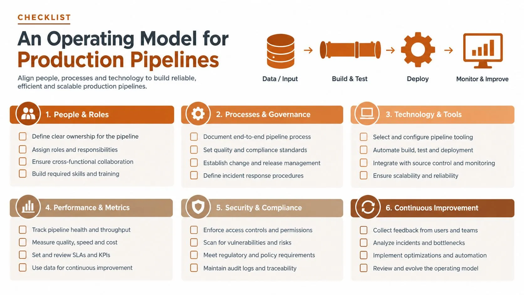
Cadence, schema, and normalization aren’t independent settings. Cadence determines which price moves you witness. Schema determines whether those moves are comparable. Normalization determines whether they can support a decision. A fast pipeline with incomplete fee fields only produces misleading answers sooner.

Begin with a minimum viable request matrix. Select the highest-value vendors, core airport and downtown locations, representative dates, and the vehicle classes that matter to the buyer. Validate that the schema captures all-in totals and fee components before adding more destinations or increasing polling frequency.

A practical first-week control loop

• Lock the dimensions: Confirm pickup and drop-off identifiers, timestamps, vehicle class, mileage policy, currency, and protection fields.
• Set regional freshness rules: Define a freshness target for each market based on observed price-change deltas, not a universal schedule.
• Measure capture quality: Review vendor-level success, cell-level fill rate, currency resolution, and missing fee fields.
• Compare stages: Check the gap between the initial headline quote and the latest available checkout total.
• Create a fallback path: Route throttled or challenge-heavy vendors to a slower queue, a browser workflow, or an approved data provider.
• Version changes: Record parser and schema versions so a new fee line or changed response structure can be traced.

A weekly review should focus on decision quality rather than request volume. If a larger scrape adds duplicate headline rates but no new all-in comparisons, reduce the frequency or redirect coverage to pickup locations, lead times, and mileage policies that remain underrepresented. Batch processing can help organize these recurring jobs, especially when collection, parsing, normalization, and delivery run on separate schedules. The batch data processing guide provides relevant implementation context.

WebscrapingHQ offers managed web data operations and custom extraction pipelines that can be configured for structured car rental fields, recurring schedules, monitoring, and delivery through formats such as JSON, CSV, S3, or webhooks. Visit WebscrapingHQ to discuss a schema-first car rental price scraping workflow built around all-in cost, regional cadence, and source-specific access requirements.